First lecture on Applied Environmental Economics honestly exceeded my expectations. Not that I had the highest expectations, but it was more interesting than I thought it would be. Partially because of the quality of the lecturer, he is quite engaging.
My laptop died halfway through the lecture, so it’s a good thing I looked over the lecture slides yesterday.
Notes
Start with Outline of Module
General admin stuff. So 2 60 minute lectures and 1 60 minute PC tutorial class per week. Consultation hours are Wednesday 10-11am and Thursday 3-4pm or we are also allowed to drop in during the employability drop in hours, so Thursday 1-3pm. I suppose not a lot of people use the employability drop ins so that’s probably why. Environmental Economics is the lecturer’s personal research area, so that should be good. I think it’s smart to pick lecturers that are actually passionate about what they teach, their lectures are a lot more motivating.
We will have some other generic seminar questions, but this is not the main focus, as we will work more on the use of Excel. The class is essentially just application of microeconomics specifically on the environment using Excel, so good transferrable skills for other applications.
This module is 100% coursework, so no summer exam (partly why I took this class ngl). There will be 4 assignments, each worth 25%. We will have 4 topics, and each topic will be underpinned with an Excel assignment.
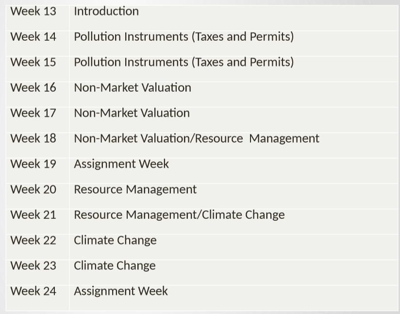
Pollution Economics – so things like taxes and permits
Non-market valuation – personally find this quite an interesting subject
Resource management – lecturer mentioned we might look at fisheries and how it ties in with Brexit. Also mentioned some historical disputes between fishing areas of the UK and Iceland
Climate change – mentioned how this is more topical over time as costs of climate change rise and have more of an impact on life.
The deadline for the submissions have been changed and can be found on SDS.
Excel based project report 1
25%
07 Feb 2020
Week 16
Excel based project report 2
25%
06 Mar 2020
Week 20
Excel based project report 3
25%
27 Mar 2020
Week 23
Excel based project report 4
25%
10 Apr 2020
Week E1
Preferred text is: Hanley N, Shogren JF and White B (2019) Introduction to Environmental Economics (3rd edition), Oxford University Press.
I have the 2nd edition from the library so that is probably what I will use. As he said, some examples may be dated in older editions, but can still be useful for basic understanding. Mine is from 2013, so not terribly dated, but I suppose it is a field that changes rapidly? This book provides background reading for each of the 4 topics we will handle in this module.
Other recommended texts, which I will probably not use but I am recording just in case I ever want to find further reading in this field:
Tietenberg T (2006) Environmental and Natural Resource Economics, 7th edn, Pearson Education (new 8th edition available)
Hanley N, Shogren JF and White B (2001) Introduction to Environmental Economics, Oxford University Press
Kolstad, C.D. (2011). Intermediate Environmental Economics (International 2nd Edition), Oxford University Press
Picture blatantly stolen from lecture slides because I cannot be bothered to write this all out
Enforceability of standards as an environmental instrument is the ease of implementation. In practice enforcement may be difficult. This can be due to arbitrary influences and where the burden of proof lies. It is important to account for the enforcement costs in the assessment of an environmental policy. The distributional impacts of a standard is uniform. All firms in the industry adhere to the same standard and there is no obvious discrimination. However, firms may face very different abatement costs. Standards also pose lower financial burden to polluters relative to environmental tax.
An example for standards in food products is that you can test a sample to make a conclusion of the total. This demonstrates the ease of implementation.
Taxes
Emissions tax has been introduced in 1920 by Arthur Pigou, where polluters pay tax based on the damage they have caused. The optimal level of pollution control is where MAC=MD. This ‘ideal’ tax is known as Pigovian Tax. Because the polluter will pay tax for each unit of pollution emitted, there is an incentive to reduce the tax they have to pay for pollution. Taxes are not as widely used as standards.
An example of environmental tax is the tax on plastic bags in grocery stores. Tax is easier to implement if the type of pollution is easy to measure.
What are the three ways in which society uses the environment?
Source of natural resources, waste sink for pollution, amenity
Q2
True or false:
A key objective of environmental economics is to ensure that the design and implementation of environmental policy reduces degradation to efficient levels.
True?
Q3
What is meant by ‘market failure’?
Defining a market failure is when a transaction between two parties have an effect on a third party that is not involved.
Q4
Using the key readings, draw a diagram that captures the three functions that the environment provides when interacting with the economy.
Eeh blah dont want to
Q5
List the four property rules
Universality/ownership // all property is privately owned and entitlements are completely specified.
Excludability/exclusivity // all benefits and costs only go to the owner of the resource
Transferability // property rights are transferable from one owner to the other
Enforceability // property rights are safe from being seized – violation of property rights result in penalties.
Q6
True or false:
In general an environmental good such as a natural forest will be overused if the resource is not privately owned.
Lecture 2: Household Surveys and Empirical Methods I
Examples of some modern household surveys:
Indian National Sample Survey (NSS) 1950
Malaysian Family Life Survey 1976-1977
World Bank Living Standards Measurement Study (LSMS) Surveys
Work began under Robert McNamara in 1979
The first LSMS surveys were in Peru and Cote d’Ivoire in 1985. The purpose of these surveys is to measure living conditions, compare the poverty rates across countries and to investigate the relationship between poverty and growth.
LSMS Surveys
Living Standards Measurement Study (LSMS) Surveys that are conducted by the World Bank or other comparable surveys that are conducted by national governments are presently available for a wide range of countries.
The surveys generate relevant data for policy makers and the research community. It is a response to a perceived need for policy relevant data that would allow policy makers to move beyond simply measuring rates of unemployment, poverty, and health care use, for example, to understanding the determinants of these observed social sector outcomes.
The Content of Household Surveys
The main components are the household questionnaire, the price questionnaire, and the community questionnaire.
The household questionnaire consists of:
Household composition, housing, fertility
Education, health, economic activities
Food expenditures, durable goods expenditures
Other income sources including remittances, saving, assets, credit markets
Anthropometric measures
Vocab: Anthropometric –
The sampling uses a two stage sample design. Clusters are selected at the first stage of the design. A cluster can correspond to a community or village. In the second stage, households are picked from each selected cluster. This two stage sample design lowers the costs of collecting data, it facilitates revisits, and makes it a lot more worthwhile to collect community data.
Stratification is the sampling within specifically targeted groups of interest to the researcher.
Vocab: Stratification –
Sample weights are used to ensure that the sample is ‘representative’ of the population.
Household Surveys versus Census
A population census covers the entire population by definition. The data obtained in a census is much less detailed than the data obtained from the household survey. Because conducting a census is much more costly, it is conducted much less frequently than household surveys. For example a census can be conducted once every 10 years. The data collected from the census can be of use to a large variety of studies and still be effective compared to household survey data. The data from the census can also be used to cross-validate the data gathered from the household survey.
I missed this lecture but went over slides before on the 16th of January. I am writing these notes on the 23rd of January before my next lecture in this module.
There will be 11 lectures in total, including this one. The readings for each week can be found in the module outlines. It is advised to do some of the reading before the lectures every Friday.
There are 5 seminars in total, so alternating every other week. I am in group 02 meeting Fridays between 15:00-16:00. We will be solving problem sets during the seminars.
We will be reading chapters from the textbook Development Economics by Debraj Ray, which is the same book we have used in the Development Economics module in the autumn term. Additionally, we will read from journal articles, chapters from the ‘Handbook of Economics’, and other books. This can all be found in the module outline on Moodle.
There will be 2 assignments, due in Week 18 and Week 22, which are supposed to provide essay-style answers to a number of questions. Each assignment is worth 10% of the final mark of this module. The assignment questions will be posted on Moodle 3 or 4 weeks before each of them is due.
– note the deadlines given in the module factsheet are different, (week 20 and week 24). Which one is right? –
The final assessment is the summer exam in May which will count for 80% of the final mark. The final exam will also require essay-style answers. The approach to the final exam will be similar to the approach used to answer the assignments. Use the assignments to prepare for the work during the exam. Learning to be comfortable with the assignments will make you more comfortable with the final exam questions. On Moodle, there are some sample questions for the final exam.
What is meant by the ‘Microeconomics of Development’? The autumn term ‘Development Economics’ class is not a prerequisite for this module, but it is useful as a reference. Traditionally the field of development economics is macro-based. Economic growth or industrialisation (sectoral transformation) are traditional measures of development. With these factors as measures of development, typical policy targets are investment and (international) trade. The instruments used in these policies include adjustments to interest rates, exchange rates or taxation.
By contrast, microeconomics of development is concerned with welfare, constraints and choices at the individual level. It looks at the incidence of poverty or life expectancy as measures of development, instead of growth and industrialisation. In this situation health and education are policy targets. Health and education have a more direct relationship with poverty.
In this module we are assessing:
The quality of life of individuals
The constraints they face and the choices they make that prevent them from improving their own situation
Policies and programmes that can have a positive impact, by removing those constraints or enabling individuals to make better choices
These changes in choices individuals are making can also have an effect on the macro level of development, like an increase in the savings rate and investment in the economy as a whole.
Outlines of lectures. (In the module outline you can find a description of each topic and reading assigned to each topic):
1. Economic Lives of the Poor
This topic is continued further in this lecture.
2. Household Surveys
3. Empirical Methods
In recent years, we have been able to obtain more data regarding choices on the micro level, as opposed to only having macro data in the past.
4. Market Failure
5. Financial Markets
6. Land and Labour Markets
7. Risk and Strategies for Coping with Risk (Insurance Markets)
These next 4 lectures are about the theory behind how we understand the poverty in developing countries, which generally revolves around market failures. Each lecture will be about market failures regarding a specific factor of production. We will also discuss the implications of market failures and the policies used to address these issues.
8. Individual Behaviour under Poverty
9. Gender and Decision-Making within Households
10. Social Networks
11. Culture and Institutions
The last 4 lectures are about decision-making and social interaction at different levels of an economy or a society. Behaviour and decision-making might be different under poverty. The implications of decision-making within households on poverty and inequality. Furthermore we will look at social networks, so groups of people who don’t live together, but are socially connected and what kind of social interactions they have and the implications of economic decision-making, why they should be taken into account when creating policy. The final topic is about shared culture or beliefs and how they affect economic decision-making and its influence on development.
When there are no market failures, the different social levels don’t have as much of an effect on decision-making in developing countries relative to developed countries. Because there are market failures, we need to be aware of the various effects of each topic.
The aim is to understand the causes and possible prescriptions for poverty.
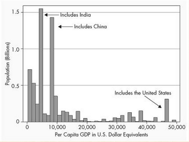
The topic of this lecture is the economic lives of the poor. To start with a description of the lives, we should note that there are large variations between average income levels across different countries in the world.
The diagram shows that a large majority of the world population makes on average 10000 per capita GDP in USD, and this is mainly driven by the extremely large populations in India and China. There is also a substantial level of people that makes more on average and this group is mainly driven by the large population of the United States.
However, it is important to note that even in countries where the average per capita is very high, there will still be a significant amount of the population making less than the country’s average, as there can be a high disparity in incomes within a single country.
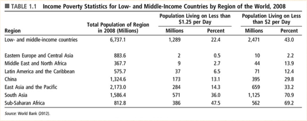
To be able to determine how many poor people live in what countries economists use various measures of poverty based on the amount of spending per person per day. This is because just using average income does not show the income disparity within a country. A Poverty Count is based on a specific income threshold and a measure of the extent of poverty.
The definition of living in extreme poverty uses a threshold of 1.25 USD per day, while moderate poverty uses a threshold of 2 USD per day. These thresholds will vary over time.
Looking at the poverty head count gives a different view than just looking at average GDP per capita in a country.
For example we can observe this discrepancy by comparing South Asia and Sub-Saharan Africa. The average GDP per capita in South Asia is a lot higher than that of Sub-Saharan Africa, yet the poverty head count percentage of these regions are quite similar and in fact South Asia has almost double the total amount of people living in moderate poverty. We can conclude that income inequality and the size of a population has an impact on how we will view poverty.
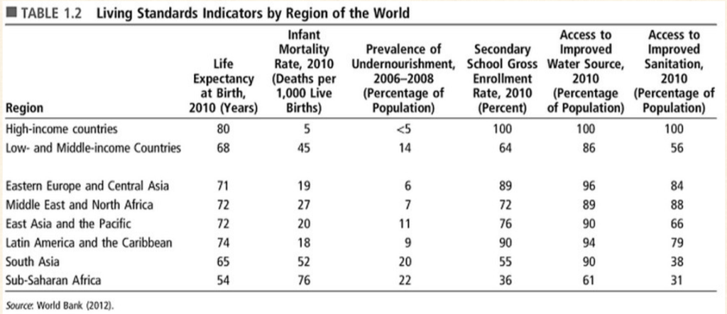
This gives us a slightly better picture of where poor people live, but more factors need to be considered. One reason for this is that having the same level of income does not necessarily equal the same quality of life in different regions of the world and people may have vastly different experiences regarding accessibility to health services, education, sanitation, etc. Additional living standards indicators need to be included to give a more accurate picture.
Countries can again have similar average GDP rates and similar poverty head count rates, but vary according to these living standards indicators.
Levels of malnourishment are quite similar for South Asia and Sub-Saharan Africa, while the average GDP per capita rates are quite different.
Another example can be seen when we compare Eastern Europe and Central Asia with Latin America and the Caribbean. The latter has a high poverty head count rate in comparison to the former, but in actuality the quality of life might not be as different as we might initially assume, because we can see that the living standards indicators are quite similar.
It is important to note that the thresholds we have for poverty head counts are just an average over a period of time. It does not mean that an individual will have that amount to spend every day. It is possible that some days their spending is zero.
What does it mean to live under the poverty threshold? What are the constraints that these people face?
Questions about Economic Lives
Economic lives of the poor in developing countries are very different from well-off individuals from richer countries, but we start by asking the same basic questions. The fundamental economic questions to understand their economic lives are the same, which might be a very different approach than for example in anthropology.
Some questions to consider:
How do they earn a living?
Do they hire out labour?
Engage in home production? Do they participate in the market?
Act as entrepreneurs?
What productive assets do they use in making a living?
How do they obtain these assets?
How do they protect themselves from adverse shocks? E.g. bad weather, poor health?
How do they save for the future?
Make provisions for their old age?
Who do they transact with? E.g. to sell their produce, or hire labour out, or obtain credit, or raw materials for production?
Journalists and travel writers may draw up a portrait which can address some of these questions, but it might not be a good representative. How would we know if this particular story is exceptional or ordinary? It might still be a very accurate account of a single case which can be useful, but might not be relied on if you want to create policy for a larger group.
Household surveys are much more useful if you want data that is a good representation of the population. It collects detailed information on a representative sample of households, including characteristics of household members, employment, assets, consumption, production etc. and may be used to make general assumptions about the population.
Banerjee and Duflo (2006) “The Economic Lives of the Poor”
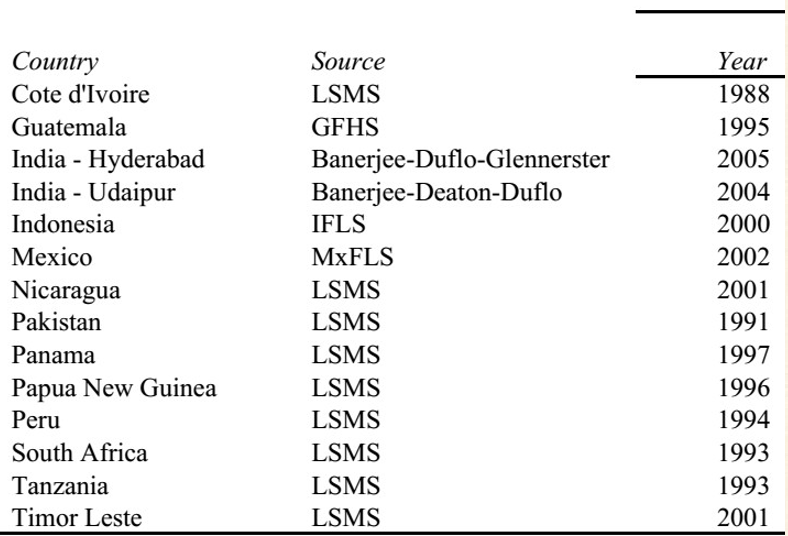
Application: Banerjee and Duflo (2006) use household surveys from 13 different countries to present a detailed portrait of the economic lives of the poor comparing living on less than $2 and $1 a day
http://economics.mit.edu/files/530 is encouraged to read, as it is not a very technical paper and should not be too difficult to understand.
These researchers shifted the focus of developmental economics to how to address poverty. The analysis was based on 14 household surveys listed below with the focus on the ‘extremely poor’ with an average per capita consumption of 1.08 USD per day and the ‘poor’ with an average per capita consumption of 2.16 USD per day (using 1993 PPP exchange rate).
“the average person living at under $1 per day does not seem to put every available penny into buying more calories. Among our 13 countries, food typically represents from 56 to 78 percent among rural households, and 56 to 74 percent in urban areas”
Given that they do not have a lot to spend, you might assume that they would use a higher percentage of their resources to improve their calorie intake, but this is not what we find. In some of these countries a substantial percentage of their budget actually goes to tobacco and alcohol, which we assume to be non-essential for their health and nourishment.
“The extremely poor in rural areas spent 4.1 percent of their budget on tobacco and alcohol in Papua New Guinea, 5.0 percent in Udaipur, India; 6.0 percent in Indonesia and 8.1 percent in Mexico; though in Guatemala, Nicaragua, and Peru, no more than 1 percent of the budget gets spent on these goods”
This is all for individuals with a budget of under $1 a day on average.
“… it is hard to escape the conclusion that the poor do see themselves as having a significant amount of choice, and choose not to exercise it in the direction of spending more on food”
Can market forces correct for market power of a monopolist?
What should government intervention be?
Monopolies and Price Discrimination: a way to extract more consumer surplus
Two-part tariff pricing scheme – working through an example
What are the welfare effects of price discrimination
Standard definition of price discrimination is to sell a product while charging different prices to different consumers. However, an application of price discrimination could be first class or business class seats on an airplane or hardcover and paperback books, where the price is corrected for the cost that is associated with the product differentiation. Using price discrimination, a monopolist may be able to increase profits without a further decrease in social welfare by charging price inelastic consumers (business people) more than price elastic consumers (students).
Can market forces alone reduce market power?
Coase (1972) Durable goods monopolist. See example in textbook. The durability of
The monopolist charges P=MC. Is there a way to restore market power?
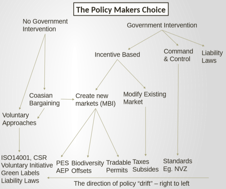
Recap of lecture slide [14] with emphasis on that we will focus on aspects like creating new (permit) markets.
Criteria to Evaluate Pollution Instruments
The policy instruments we will be looking at are taxes, standards, and permits. We will use four criteria to evaluate these policy instruments.
Cost-effectiveness and economic efficiency
Fairness
Dynamic Efficiency
Enforceability
Cost-Effectiveness and Economic Efficiency
Cost-effectiveness means that outcomes are maximised with the given resources or to achieve a given outcome with minimum resources.
The difference between economic efficiency and cost-effective policy is that one is a theoretical ideal that firms may strive for, but is not realistically achievable, while the other is the more practical goal that firms try to achieve.
The best practical policy would create output and emission at economic efficiency – marginal damage equals marginal abatement cost.
Economic efficiency – MD = MAC
This is hard to achieve, because the exact locations of MAC and MD are generally not known. So an environmental policy is considered in terms of cost-effectiveness over economic efficiency, meaning that given the resources the policy aims to achieve maximum environmental improvement or to set an amount of environmental improvement for the least cost.
Fairness
Welfare economics deals with the concept of ‘fairness’ and how government policies could be evaluated on the grounds of fairness. This field deals with normative questions, so value judgements, instead of positive questions that are just factual.
The implication here is that fairness is based on value judgements. Because it is subjective, it is difficult as a criteria. An environmental tax might be considered to be regressive when the resources collected by the tax gets distributed again. Is this a fair tax? Will everyone agree on whether it is fair or not?
Polluter Pays Principle (PPP)
The Polluter Pays Principle (PPP) is a basic principle of environmental policy, which states that the polluter is the one who should pay for the damages from the pollution that they created. – PPP (OECD, 1972)
The premise is that public measures, read government intervention, are necessary to reduce pollution and achieve better allocation of resources. It can also achieve better allocation of resources by ensuring that the price of goods reflect more accurately their relative scarcity depending on the quality and quantity of environmental resources. Economic agents should act according to price increases.
Fairness as a criteria of policy instruments relates to financial consequences, but also the resulting environmental effects. For example, the equality of environmental exposure to pollution, situational fairness by preventing changes in environmental quality that might result from a change to the local environment, such as a new industrial plant.
Historically the OECD advocated the Polluter Pays Principle (PPP) for the correction of negative externalities in industries with market failures.
Some variations of this principles exist that better reflect other forms of market failure. We will be studying the Provider Gets Principle (PGP), the Beneficiary Pays Principle (BPP), and the User Pays Principle (UPP). The use of any of these principles will be based on the value judgement of the policy makers.
A simple example in the EU is that we currently offer farmers various payments for providing environmental goods and services via the Common Agricultural Policy (CAP). The UK has some foundations for such policy initiatives.
Do farmers actually supply or destroy environmental goods and services?
A ‘reference point’ has been established that views current actions as provisions – so as PGP, not PPP. The provider – the farmer – gets paid for supplying the environmental resources, instead of polluters paying for the damages to the environment.
This value judgement matters, and it frames the resulting policy design and implementation (political discourse).
The PGP might be applicable to the UK post-Brexit regarding how the country will handle agricultural policy.
References to political economy and what is and is not considered to be a public good.
Dynamic Efficiency
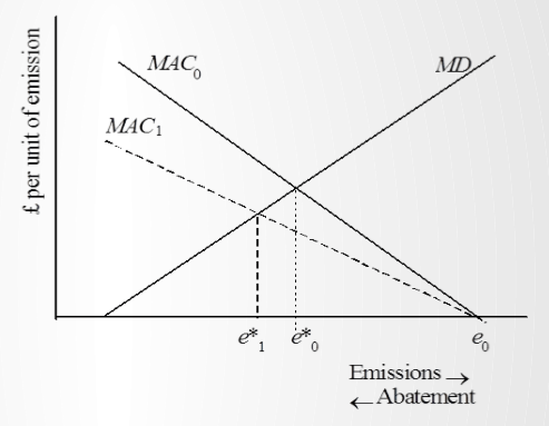
Dynamic efficiency is having investment in new and/or improved abatement technology.
MAC moves from 0 to 1 with the introduction of new technology. The point e* illustrates the optimal level of pollution. A policy with dynamic efficiency provides dynamic incentives to reduce abatement costs to MAC1 with the introduction of a new and more efficient technology. The optimal level of pollution e* falls from 0 to 1.
The policy preferably encourages firms to adopt new technology, because innovation reduces the optimal level of pollution.
Enforceability
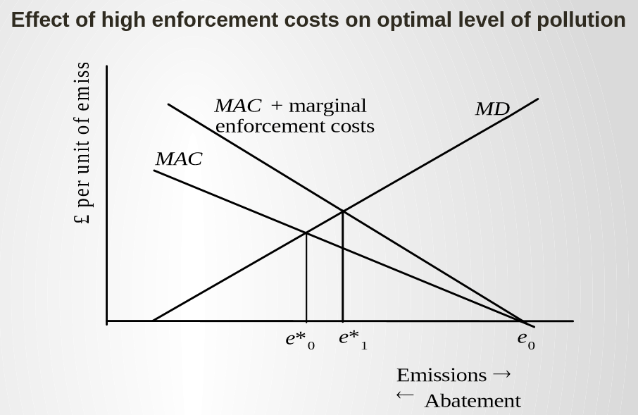
There is no point in introducing a new environmental policy if it is very difficult to enforce. Complex environmental schemes can be difficult and costly for regulatory bodies to observe and check whether polluters are complying.
The cost of enforcement should be taken into consideration in any assessment of environmental policies. High enforcement costs increase the optimal level of pollution.
High enforcement costs increase the optimal level of pollution e*.
Standards
Standards are the most common approach of government intervention. Some types of standards are the following:
Ambient quality – examples are the maximum noise level at workplace or air qualities in cities.
Emissions – examples are a standard set on the maximum emissions of sulphur dioxide or emission standards for cars.
Product – an example is a standard set for pesticide residue in food or drinking water.
Process – a standard for a certain type of release valve in the in the production of polyethylene.
Input – standards on the maximum content of sulphur in coal or restrictions imposed on the use of fertilisers in water protection zones.
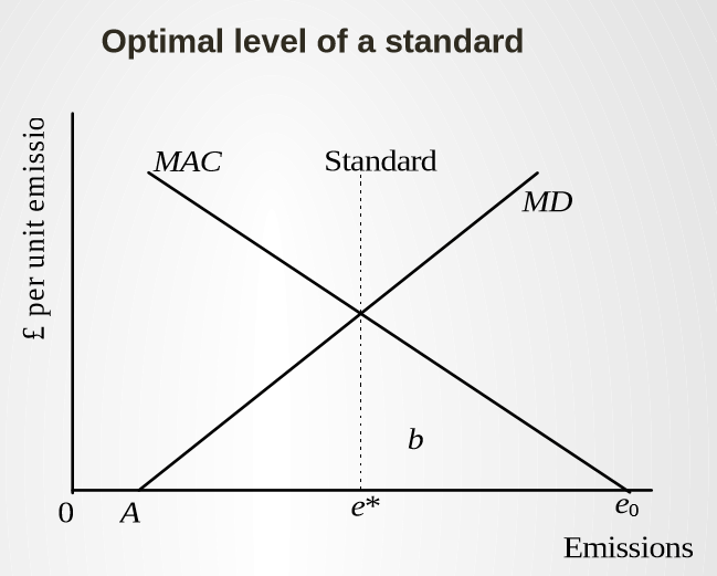
Initial level of emissions is e0, while e* is the optimal level of pollution. Segment 0A shows the emissions assimilated by the environment.
Question: What is the cost to the polluter if a standard is set of e*?
Answer: Polluters incur costs equivalent to the area under the MAC, area b, in order to reduce their emissions e*.
In practice there are some issues with setting an optimal standard. The exact positions of MAC and MD are unknown. The MAC differs between polluters, meaning that there is a separate optimal level of pollution for each individual polluter.
MACi=MD
A standard sets an average MAC=MD, but standards do bring certainty to hit policy goals.
Standards do not achieve the reduction of pollution cost effectively. This is because different polluters face different MAC.
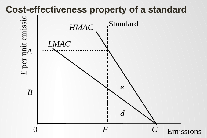
Assume the two different polluters start at point C with the same initial level of emissions. The two curves are firms with high (HMAC) and low (LMAC) abatement costs. A regulatory body sets a standard for the industry for emissions at point E. Both firms need to adhere to point E.
Question: What abatement costs are incurred by the two firms?
LMAC faces a lower cost, area d. HMAC faces a higher cost, area d + e. The total industry costs of meeting the standard are 2d + e (because we are looking at an example of an industry with only two firms for simplicity). It can be perceived as fair treatment, because they face the same standard. However, HMAC incurs considerably higher costs than LMAC in order to meet the standard.
Why is a standard not cost-effective?
For cost-effective outcome, MAC needs to be equal for the two firms (or all firm in the industry if we apply it to real world examples). With the standard set at E firm HMAC pays A per unit emission, while firm LMAC pays B per unit emission.
Consider that if HMAC produces one less unit of pollution, LMAC can abate one additional unit of pollution and the industry emission level would be unchanged. Since we are looking at marginal costs, HMAC would save abatement costs (cost A) and LMAC would incur additional costs (cost B). Since A>B, this would result in net cost saving across the industry. Therefore having a industry standard is not cost-effective. To make it cost-effective, continue until the marginal costs in the industry are equal, where HMAC=LMAC. This condition for cost-effectiveness is known as the equi-marginal principle.
– End of lecture notes for lecture 3, continue slides another day –
Hanley N, Shogren JF and White B (2013) Introduction to Environmental Economics, Oxford University Press
Chapter 1 provides a good introduction to the topic area and how the environment and the economy interact. There are also some more advanced topics covered that relate to how the economy and environment interact.
Introduction to Environmental Economics
Part I: Economic Tools for the Environment
1. Introduction: Economics for the Environment
Outline of this chapter:
Discuss the connections between the economy and the environment.
Review ten key insights from environmental and resource economics that environmental scientists, managers, and politicians ought to be aware of.
Explain how this book is best used.
Provide an overview of happens in the rest of the book.
1.1 The Economy and the Environment
The relationship between economics and environmental and natural resource policy is important due to the ‘unpriced’ or non-market services that the natural environment provides. The value of protecting wetlands for their biodiversity, flood defence, and pollution treatment functions is as economic of a value as the production of oil from an oilfield.
It might be beneficial to appreciate how the economy and the environment are interlinked through dynamic interactions.
First, the environment provides the economic system with inputs of raw materials and energy sources for production. Resources can either be non-renewable – coal or iron ore – renewable – such as fisheries or forests.
Second, the use of the environment as a waste sink. Waste may come from production or consumption. It comes in a number of basic types: solid, air- or waterborne. The environment has a limited assimilative capacity to absorb and transform waste into harmless substances. Pollution can be seen as when emission exceeds assimilative capacity and produce some undesirable impact.
Third, it provides households with amenity, from which they may derive utility (happiness, satisfaction).
Finally, it provides the economic system with basic life-support services.
Information about the upcoming assessment will be posted sometime next week. Students will have about 2 weeks (1,5 weeks really) to do the assignment. Each assignment should be about 1000 words. All problems will be similar to those done in workshops. [So go to the workshop. pls]
Started with a continuation of lecture slides 1 as we did not fully finish this in the previous lecture.
Notes
Lecture 1 – Introduction
Continuation on slide [21], on seeing the environment as a waste sink.
The physical assimilative (read absorbing) capacity of the environment can be categorized under land, water, and atmosphere. It is determined by physical factors eg climate, rainfall, wind patterns and geographical location. We can distinguish between degradable waste and cumulative waste. For cumulative waste we have to consider the importance of the threshold of the environment as a waste sink.
If we consider cumulative waste and there is a threshold, we can avoid reaching this threshold using economic instruments.
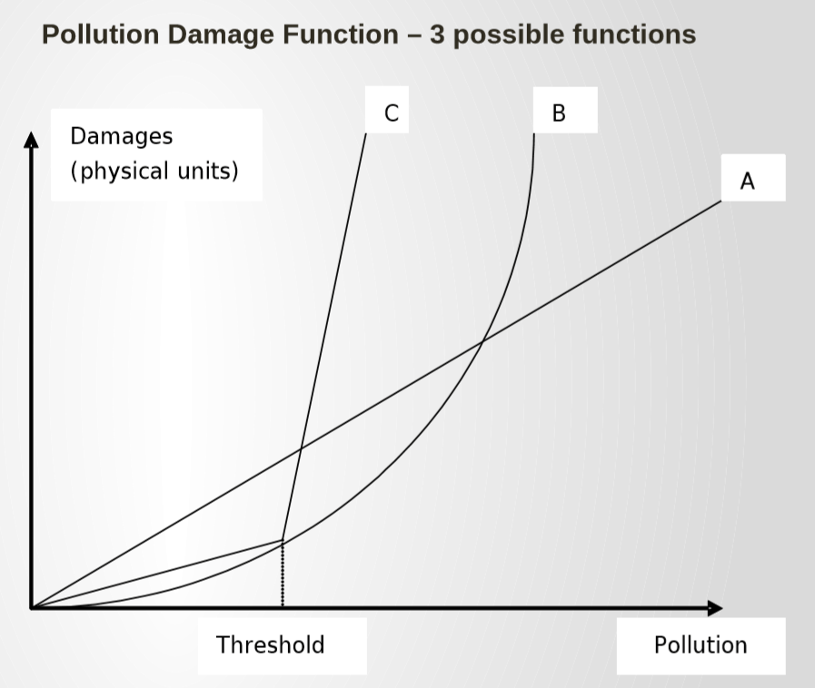
Taken from the slides
This diagram illustrates 3 possible functions of pollution damage. Damage function A is linear. Damage function B is exponential. Damage function C is a function with a kink, at which the threshold is. The point as which the kink is, is the point at which the marginal damages caused by pollution become larger. So after the threshold, the cost in damage caused by pollution becomes higher than the cost in damage caused by pollution before the threshold.
An example is the level of oxygen in water (BOD). If it falls below a particular level due to water pollution it becomes extremely dangerous to aquatic species, like a threshold.
We can describe the assimilative waste capacity of the environment in a mathematical way:
Stock of degradable pollutant (S) at time t is given by S = F – A
Stock of cumulative pollutant (S) at time t* is given by S = ΣF
F represents the positive flow (of pollution) in a year. A represents the amount of pollution that is assimilated by the environment in a year.
We might need to take efforts in environmental management to prevent further pollution as to avoid the threshold.
Recycling
The 3R’s of recycling are Reduce, Reuse, Recycle. After this, the final option is to dispose. There are limits to Reusing and Recycling, partly due to the laws of thermodynamics, but also the costs associated with re-use and recycle.
First lecture for Industrial Economics. The lecturer seems fun. She finds a lot of personal examples about how market failures have failed her. She seems to repeat the same thing a few times, which is honestly quite useful in lectures. Did not make notes before the class started.
This class seems very “traditionally” economics, as in the focus on firms. Most of my specialisations in stage 3 moved away from that, so it might be nice to refocus.
Notes
Introduction to the module, admin notes
This is the second year this module is taught at this university by her, but she taught this subject in various other universities.
Some points she included to be motivational I suppose:
Students who learn with the mindset: “Work hard to learn more and get smarter.” Get higher marks and have better test scores.
Dweck, C. Mindset: The New Psychology of Succsess (Random House, 2006).
This reminds me of this thing we read in the psychology textbook for the IB, about how people who think intelligence is a fixed trait tend to not perform as well, while people who believe intelligence is a skill you nurture and develop perform better on average. It is kind of evident that this link exists I suppose, but sometimes it can be beneficial to really point this out.
Focus on your improvement.
Of course.
Then some notes on how you are not here to learn to imitate well, but to learn the method and how to apply it to other situations. Which is why they will not give us the answers to past paper questions.
The point of this module: Industrial Economics is really just an application of microeconomic theory. Specifically on the analysis of firms, markets and industries where competition is less than perfect. – Because perfect competition is a theoretical concept and it does not exist in the real world. Therefore these skills may be transferable to other applications of microeconomic theory.
The overall aim is to provide a framework for explaining firm behaviour, assessing the welfare consequences of this behaviour and discussion policy prescriptions.
This module will be of interest to people who want to pursue careers as firm managers, consultants, and policy makers. As a policy maker you need to assess the competitiveness of an industry and make decisions based on whether you wish to increase or decrease it (wanting to decrease competitiveness is rare). As a consultant you may need to advise management about the best strategic behaviour in a specific market setting. As a manager you may want to undertake that strategic behaviour.
It is relevant to the study of other disciplines in economics, like Macroeconomics or International Economics, as the behaviour of firms affects the performance of the economy both domestically and internationally.
Learning outcomes:
Ability to explain how firms’ decisions regarding price, advertising and R&D etc. can be modelled and evaluate the impact of those decisions on the structure and performance of markets.
Understand and apply the basic concepts of game theory to the analysis of firm’s strategic behaviour.
Identify the implications of the theory for the design and implementation of industrial policy.
Ability to follow the analysis of economic problems, construct your own economic arguments and offer critical comments on the arguments of others.
The assessment for this module consists of two components. Coursework (20%) and the final exam (80%).
The coursework is divided over an ICT in week 8? (8%) due Tuesday 03 March 2020 week 20, participation in seminars when covering the problem sets (4%), and a 1500 word essay (8%) due 30 March 2020 (week 24). The essay questions are already available on the module outline.
I have looked at the module outline for this class. It is super extensive and detailed. I should refer back to it often, it should be very helpful.