20/01/2020 Monday 15:00-16:00
Lecture continued on lecture slides 2, from slide [14] until [31]. We still have not finished lecture slides 2.
Notes
Lecture 2 – Topic 1: Environmental Pollution (continued)
Recap of lecture slide [14] with emphasis on that we will focus on aspects like creating new (permit) markets.
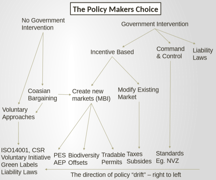
Criteria to Evaluate Pollution Instruments
The policy instruments we will be looking at are taxes, standards, and permits. We will use four criteria to evaluate these policy instruments.
- Cost-effectiveness and economic efficiency
- Fairness
- Dynamic Efficiency
- Enforceability
Cost-Effectiveness and Economic Efficiency
Cost-effectiveness means that outcomes are maximised with the given resources or to achieve a given outcome with minimum resources.
The difference between economic efficiency and cost-effective policy is that one is a theoretical ideal that firms may strive for, but is not realistically achievable, while the other is the more practical goal that firms try to achieve.
The best practical policy would create output and emission at economic efficiency – marginal damage equals marginal abatement cost.
Economic efficiency – MD = MAC
This is hard to achieve, because the exact locations of MAC and MD are generally not known. So an environmental policy is considered in terms of cost-effectiveness over economic efficiency, meaning that given the resources the policy aims to achieve maximum environmental improvement or to set an amount of environmental improvement for the least cost.
Fairness
Welfare economics deals with the concept of ‘fairness’ and how government policies could be evaluated on the grounds of fairness. This field deals with normative questions, so value judgements, instead of positive questions that are just factual.
The implication here is that fairness is based on value judgements. Because it is subjective, it is difficult as a criteria. An environmental tax might be considered to be regressive when the resources collected by the tax gets distributed again. Is this a fair tax? Will everyone agree on whether it is fair or not?
Polluter Pays Principle (PPP)
The Polluter Pays Principle (PPP) is a basic principle of environmental policy, which states that the polluter is the one who should pay for the damages from the pollution that they created. – PPP (OECD, 1972)
The premise is that public measures, read government intervention, are necessary to reduce pollution and achieve better allocation of resources. It can also achieve better allocation of resources by ensuring that the price of goods reflect more accurately their relative scarcity depending on the quality and quantity of environmental resources. Economic agents should act according to price increases.
Fairness as a criteria of policy instruments relates to financial consequences, but also the resulting environmental effects. For example, the equality of environmental exposure to pollution, situational fairness by preventing changes in environmental quality that might result from a change to the local environment, such as a new industrial plant.
Historically the OECD advocated the Polluter Pays Principle (PPP) for the correction of negative externalities in industries with market failures.
Some variations of this principles exist that better reflect other forms of market failure. We will be studying the Provider Gets Principle (PGP), the Beneficiary Pays Principle (BPP), and the User Pays Principle (UPP). The use of any of these principles will be based on the value judgement of the policy makers.
A simple example in the EU is that we currently offer farmers various payments for providing environmental goods and services via the Common Agricultural Policy (CAP). The UK has some foundations for such policy initiatives.
Do farmers actually supply or destroy environmental goods and services?
A ‘reference point’ has been established that views current actions as provisions – so as PGP, not PPP. The provider – the farmer – gets paid for supplying the environmental resources, instead of polluters paying for the damages to the environment.
This value judgement matters, and it frames the resulting policy design and implementation (political discourse).
The PGP might be applicable to the UK post-Brexit regarding how the country will handle agricultural policy.
References to political economy and what is and is not considered to be a public good.
Dynamic Efficiency
Dynamic efficiency is having investment in new and/or improved abatement technology.
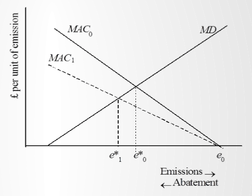
MAC moves from 0 to 1 with the introduction of new technology. The point e* illustrates the optimal level of pollution. A policy with dynamic efficiency provides dynamic incentives to reduce abatement costs to MAC1 with the introduction of a new and more efficient technology. The optimal level of pollution e* falls from 0 to 1.
The policy preferably encourages firms to adopt new technology, because innovation reduces the optimal level of pollution.
Enforceability
There is no point in introducing a new environmental policy if it is very difficult to enforce. Complex environmental schemes can be difficult and costly for regulatory bodies to observe and check whether polluters are complying.
The cost of enforcement should be taken into consideration in any assessment of environmental policies. High enforcement costs increase the optimal level of pollution.
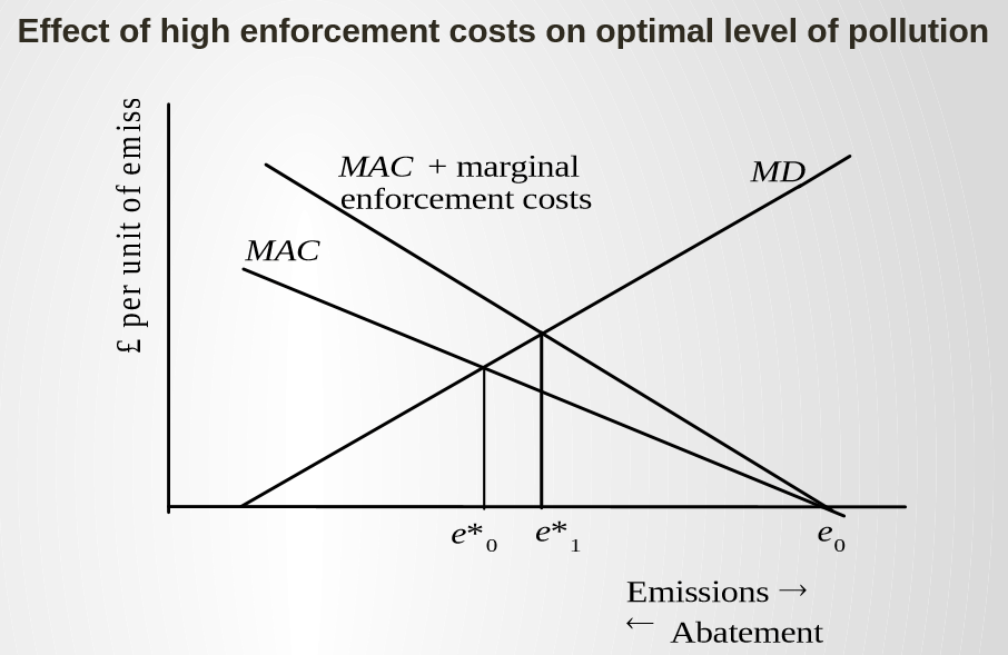
High enforcement costs increase the optimal level of pollution e*.
Standards
Standards are the most common approach of government intervention. Some types of standards are the following:
- Ambient quality – examples are the maximum noise level at workplace or air qualities in cities.
- Emissions – examples are a standard set on the maximum emissions of sulphur dioxide or emission standards for cars.
- Product – an example is a standard set for pesticide residue in food or drinking water.
- Process – a standard for a certain type of release valve in the in the production of polyethylene.
- Input – standards on the maximum content of sulphur in coal or restrictions imposed on the use of fertilisers in water protection zones.
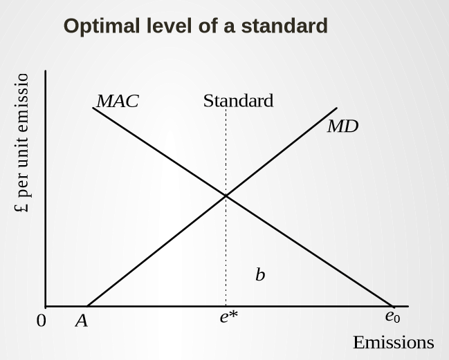
Initial level of emissions is e0, while e* is the optimal level of pollution. Segment 0A shows the emissions assimilated by the environment.
Question: What is the cost to the polluter if a standard is set of e*?
Answer: Polluters incur costs equivalent to the area under the MAC, area b, in order to reduce their emissions e*.
In practice there are some issues with setting an optimal standard. The exact positions of MAC and MD are unknown. The MAC differs between polluters, meaning that there is a separate optimal level of pollution for each individual polluter.
MACi=MD
A standard sets an average MAC=MD, but standards do bring certainty to hit policy goals.
Standards do not achieve the reduction of pollution cost effectively. This is because different polluters face different MAC.
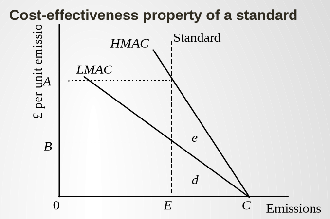
Assume the two different polluters start at point C with the same initial level of emissions. The two curves are firms with high (HMAC) and low (LMAC) abatement costs. A regulatory body sets a standard for the industry for emissions at point E. Both firms need to adhere to point E.
Question: What abatement costs are incurred by the two firms?
LMAC faces a lower cost, area d. HMAC faces a higher cost, area d + e. The total industry costs of meeting the standard are 2d + e (because we are looking at an example of an industry with only two firms for simplicity). It can be perceived as fair treatment, because they face the same standard. However, HMAC incurs considerably higher costs than LMAC in order to meet the standard.
Why is a standard not cost-effective?
For cost-effective outcome, MAC needs to be equal for the two firms (or all firm in the industry if we apply it to real world examples). With the standard set at E firm HMAC pays A per unit emission, while firm LMAC pays B per unit emission.
Consider that if HMAC produces one less unit of pollution, LMAC can abate one additional unit of pollution and the industry emission level would be unchanged. Since we are looking at marginal costs, HMAC would save abatement costs (cost A) and LMAC would incur additional costs (cost B). Since A>B, this would result in net cost saving across the industry. Therefore having a industry standard is not cost-effective. To make it cost-effective, continue until the marginal costs in the industry are equal, where HMAC=LMAC. This condition for cost-effectiveness is known as the equi-marginal principle.
– End of lecture notes for lecture 3, continue slides another day –
