Lecture 1: Monopoly
Overview of the lecture:
- Monopoly behaviour
- Social welfare under monopoly
- Efficiency of monopoly
- DWL (dead weight loss) and its determinants
- Evaluation of government intervention
Monopoly behaviour
In a monopoly, we face a downward sloping demand curve, meaning that quantity demanded falls. The standard assumed objective of a monopolistic firm is to maximise profits. In real life we might find that this objective is deviated from, like for some companies that wish to maximise sales over profits.
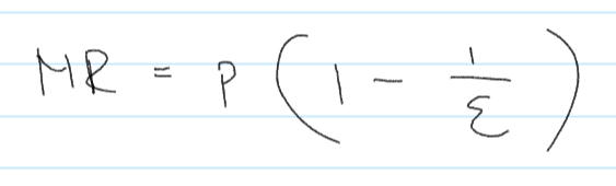
For now, we assume we wish to maximise profits. If we consider maximising profits, the optimal quantity sold is the point at which marginal revenue equals marginal cost [MR=MC]. In a monopoly, the price of the product will be above the marginal cost. How far the monopoly price is above market price depends on the price elasticity of demand.
The price elasticity of demand is the percentage change in quantity resulted from a 1 percent change in price.
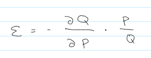
The amount of market power that a monopolistic firm can exercise can be calculated with the Lerner index.
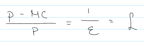
So the difference between the monopolistic price and the marginal cost at a given quantity over the monopolistic price gives the Lerner index. This is also the inverse of the price elasticity of demand. The interpretation of this is that a high price elasticity of demand for a monopolistic good decreases the market power of the monopolist. High elasticity means that consumers will switch to purchasing other goods instead of the monopolistic good with higher mark-up, which makes intuitive sense. If there is low price elasticity of demand, price does not significantly affect the quantity demanded, and therefore the monopolist can demand a higher mark-up. In this case the Lerner Index is higher, meaning that the monopolist has higher market power.
Social welfare under a monopoly
Intuitively, social welfare under a monopoly is lower compared to social welfare in perfect competition.
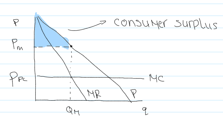
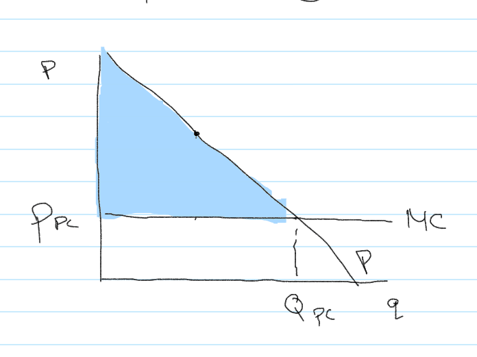
Consumer surplus (CS) is the area under the demand curve and above the price of the monopolist. Consumer surplus consists of the consumers that pay the monopolist price to buy a unit of the product, but also consumers that had a higher willingness to pay (WTP). These consumers are making an (economic) profit, therefore creating the consumer surplus. In perfect competition, the market price would be lower, and more consumers would purchase the good. More consumers will have had a higher willingness to pay. Therefore the consumer surplus would have been higher, and is relatively lower in a monopoly.
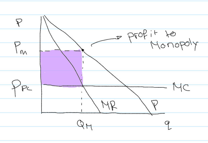
The monopolist’s profits are the price in the monopoly times the quantity sold at that price level minus the cost of production. In perfect competition there are no abnormal profits (in the long run). This is also the producer’s surplus (PS).
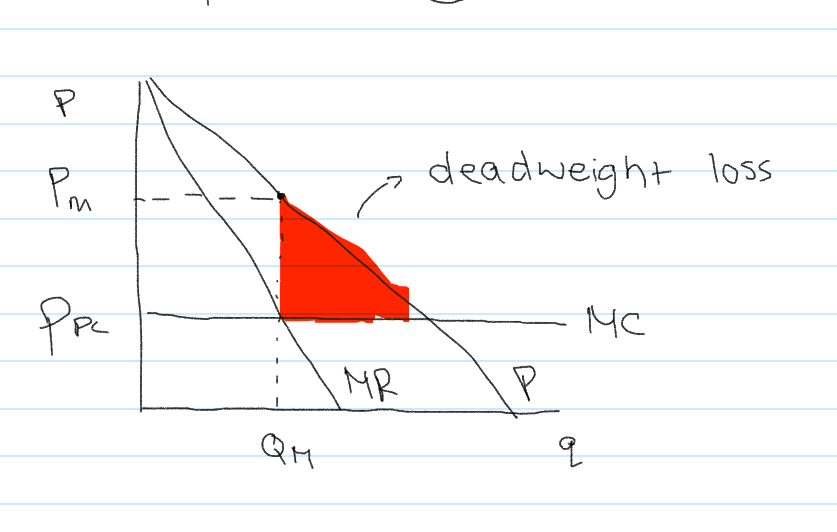
The deadweight loss (DWL) is created from missing transactions. An amount of consumers would have paid for the product at a price that would have covered the cost of production, but due to the price mark-up of the monopoly, this economic activity is lost. The DWL is lost transactions that would still have been profitable.
Eg a train ticket from London to Edinburgh. £30 might have covered the cost of a seat on the train, but the price mark up can be up to £135, due to the monopoly on public transport. Might be cheaper to fly.
In a comparison to perfect competition, social welfare is lost due to the deadweight loss created by the price mark-up that the monopolist is able to demand. In perfect competition the producer makes no (abnormal) profits. In a monopoly, the producer can “force” abnormal profits with the creation of a deadweight loss as a consequence.
Monopoly and efficiency
We can distinguish between static and dynamic efficiencies. Under static inefficiencies falls allocative and productive inefficiency:
Allocative inefficiency is the deadweight loss caused by loss of profitable transactions due to the price mark-up demanded by a monopolist.
Productive inefficiency is the loss in efficiency due to the monopolist not adopting the most efficient technology to produce. A monopolist does not have the incentives to improve their efficiency relative to producers in a perfect competition.
Dynamic inefficiency is the loss due to no incentive to introduce new (better) products or improve the process . No (or lower) incentive for innovation.
She mentioned this is an essay topic, but I can’t find it in the module outline. I think she’s mistaken or like it was an essay topic in the previous years.
Determinants of Allocative Inefficiency (DWL)
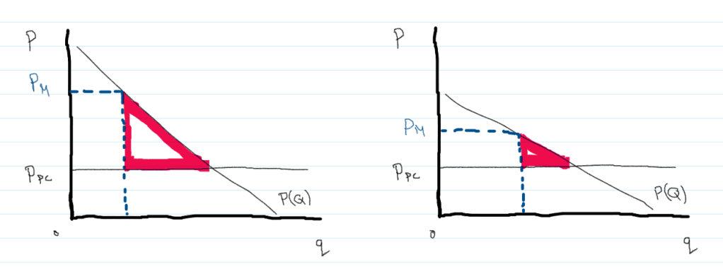
(a) Price
The monopolist’s price is always higher than the price in perfect competition. This will always create some deadweight loss. The higher the monopolist’s price is relative to the price in perfect competition, the larger the deadweight loss is in the market.
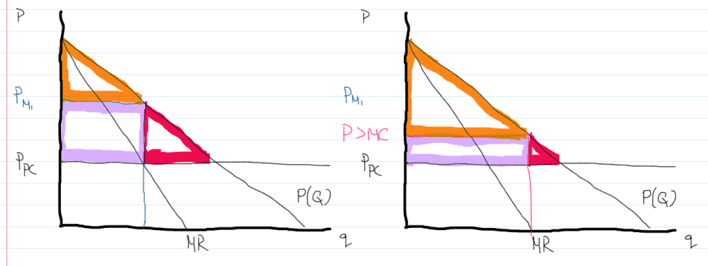
The orange area is the consumer surplus (CS) and the purple area is the producer surplus (PS). CS + PS = SW, surplus welfare. The red area is the deadweight loss (DWL). A lower monopoly price creates a higher surplus welfare and a lower deadweight loss.
The lower the price & the closer to the marginal cost (MC), the higher the surplus welfare and the lower the deadweight lost (DWL) as more consumers will now be served compared to if the price is further away from the marginal cost (MC).
(b) Price Elasticity of Demand
The elasticity of demand determines the size of the deadweight loss. If the product is relatively price elastic, then the amount the monopolist charges significantly affects the amount of output purchased. The demand curve is relatively flat. In this case, a monopolist is not able to demand as high of a mark-up on the product. When the price elasticity of a product is relatively low, or inelastic, a change in price does not really change the quantity demanded. This allows the monopolist to charge a higher mark-up without losing a significant amount of sales. The demand curve is relatively steep.
Price inelasticity allows for a higher mark-up, and greater deadweight loss. Price elasticity only allows for a slight mark-up, and so the deadweight loss is lower.
The flatter the demand curve, the more elastic the consumer respond to a price change, the lower the price markup that the monopolist can demand -> lower deadweight lost! The relationship between the price elasticity of demand and price-markup is inverse.
(c) Size of the Market
The size of the market also affects the size of the deadweight loss. If the market is small, the deadweight loss will be small too, because there will be smaller amount of total transactions in the market. So if there is a market failure, there will be less forgone transactions.
add image showing size of market and its effect on deadweight loss later.
Productive inefficiency
So if productive inefficiency is the loss in efficiency due to the monopolist not adopting the most efficient technology to product. The monopolist is inefficient because the marginal costs are higher than the marginal market costs [MCh>MC]. The monopolist’s costs are higher than a firm in perfect competition.
add diagram comparing monopolist and perfect competition Marginal Cost
Deadweight loss might appear smaller initially, but we have to consider that the price also changes. A higher Marginal Cost means that the price charged will increase, which will result in a larger deadweight loss. Less quantity is being demanded, creating inefficiency. Part of the inefficiency also comes from a lower profit per unit of the product. This also leads to a larger deadweight loss.
Monopoly and efficiency
Allocative inefficiency occurs when a monopoly undersupplies compared to the efficient outcome in perfect competition. How do we decide whether the government should intervene or not?
Productive inefficiency occurs due to managerial slack. Compare the Darwinian versus Schumpeterian effect:
Darwinian effect: Monopolies are bad for Research and Development because there is no incentive to innovate in a monopoly due to the lack of competition in the market. There is no reason to improve the product. In a truly competitive environment, only the ‘fittest’ survive, meaning that only the company that is best adapted to the industry will come out on top and produce while the others will leave the industry. In perfect competition firms must innovate and perform R&D in order to be ‘fit’ and survive.
The Schumpeterian hypothesis states that there is a close relationship between innovation and the market structure. Only companies that have market power, at the best monopolist, can support the costs. Innovation itself can itself determine a monopoly position.
From the Darwinian perspective perfect competition is the best for innovation. From the Schumpeterian perspective monopolies are better for innovation.
Schumpeter is known as the creator of the concept of ‘creative-destruction’ where firms grow and innovate and are challenged by competitors and then exit the market which is all driven by perfect competition. The strive for monopolistic power is what drives innovation and the monopolistic power itself gives the means for innovation.
Dynamic inefficiency (x-inefficiency) is the loss due to no incentive to introduce new or improve the process, so there is no (or lower) incentive for innovation. Dynamic inefficiency refers to the disincentive to introduce new products or new processes of production. It is the difference between efficient behaviour of businesses assumed or implied by economic theory and the observed behaviour in practice caused by a lack of competitive pressure.
The concept was introduced by Harvey Leibenstein (1966) but more recent examples are available, like in a paper by Hey & Liu (1997), which tests the hypothesis that rivalry reduces x-inefficiency and this is found in a sample of UK manufacturing firms in 19 UK manufacturing industries during 1970-80s. The same test is conducted for other countries such as Australia, Canada, Japan, Korea, and the US by Caves and co-authors (1992). Klette (1999) finds that plants with larger price-cost margins are less efficient in a productivity sense, compared to plants with a smaller price-cost margin, which he tested for the manufacturing sector in Norway.
Can market forces alone reduce market power?
Continued in the next lecture.
