Lecture 2 – Topic 1: Environmental Pollution
Pollution is the classic example of negative externalities. We will be modelling markets for permits using excel. Furthermore we will discuss why there is a preference for incentivizing firms’ behaviour that affect the environment through financial instruments (taxes and pollution permits) over standards.
Overview of this lecture:
- Explaining the role of property rights
- Define and explain externalities
- Determine the optimal level of pollution
- Introduce criteria to evaluate pollution instruments
- Examine standards, taxes, and pollution permits
Property Rights and the Environment
Absences of property rights (PRs) are the underlying cause of pollution. Because nobody owns the air, nobody stops anyone from polluting it, until someone claims the resource. There are 2 components in the property rights regime: property rights and property rules.
Property Rights are the rights and duties regarding the use of a resource, like the environment. A property right is a claim to a benefit stream (an income stream). These rights are typically protected in law. Reference to political economy and property rights.
Property Rules are the rules that govern the way the property rights are exercised.
Main characteristics of property rights:
- Universality/ownership – all property is privately owned and all entitlements are completely specified.
- Excludability/exclusivity – all benefits and costs accrue only to the owner of the resource, either directly or indirectly through sales or other ways.
- Transferability – all property rights are transferable from one owner to another by means of voluntary exchange.
- Enforceability – all property rights are safe from being seized or encroached upon – violation of property rights result in penalties.
These 4 characteristics of Property Rights must exist for the market to function properly. We could apply this to other externalities to work out problems with market failures.
Vocabulary: accrue – to come into existence as a legally enforceable aim / to come about as a natural growth, increase, or advantage / to come as a direct result of some state or action / to accumulate or to be added periodically.
Vocabulary: encroached – to enter by gradual steps or by stealth into the possessions or rights of another / to advance beyond the usual or proper limits.
Market failure
A market failure will occur if one or more of these 4 characteristics are not present.
- Not owned – overuse. Examples are atmosphere, common grazing land, tropical rainforest, fisheries. We will come back to this characteristic of property rights when discussing fisheries. It is a typical “open access” problem causing overfishing. We can correct the market failure by establishing ownership over properties. – Maybe relates to the South China Sea conflict. Kyoto: attempt to get countries to reduce CO2 emissions.
- Not exclusive – An application that illustrates the issue is a paper mill that discharges waste from production process into a nearby river. The costs are now being ‘shared’ by local fishermen. It has become a public cost, a third party is negatively affected.
- Not transferable – If properties are not transferable, there is no incentive for the owner of the resource to conserve it for any longer than he or she needs. The owner might exhaust the resource because there is no reason to protect or maintain it as there is no way to bring it back on the market.
- Not enforceable – if you are unable to establish private property rights, which leads to public goods, for example a beautiful landscape. But doesn’t a beautiful landscape’s economic value still get captured in the increased price of accommodation around the landscape?
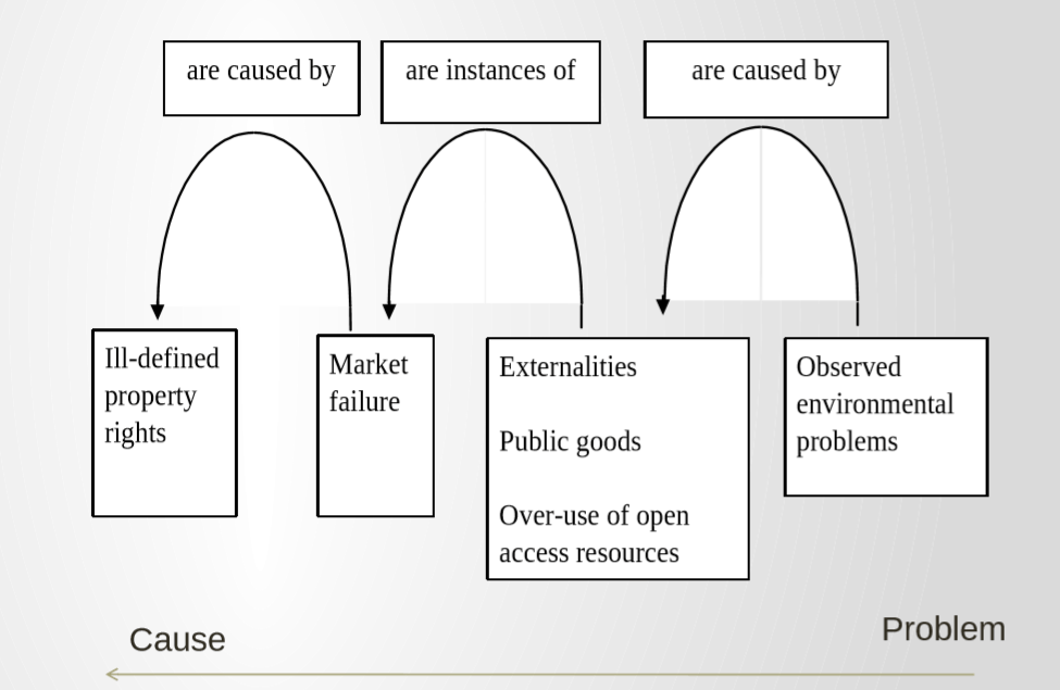
Link between property rights and environmental problems
Externalities
A typology of externalities
An externality occurs whenever an individual’s utility or production possibilities are affected by variables whose values are chosen by others, and the individual is not compensated for (or pays for) the cost (or benefit).
Baumol and Oates (1988), Page 17.
There are different types of externalities. We have already discussed positive and negative externalities, basically if the effect on the third party is seen as a cost or as a benefit. There are also cumulative or non-cumulative externalities, whether it gets assimilated by the environment or if it aggregates. Another way to differentiate is between point or non-point externalities, which is the difference in whether you can clearly see the source of the pollution. Visible smoke is an example of a point externality as we can pinpoint the polluter easily, while water pollution is an example of a non-point externality, because the source of the pollution is not always clear. Furthermore we have regional or global externalities, and continuous or episodic externalities.
We also differentiate between whether the externality is created by the consumption or the production of a transaction.
Externalities do not require to have physical linkages – an example might be how Europeans can be concerned about whale hunting or deforestation of the Amazon rainforest. These concerns are not reflected in the costs or benefits of an economic activity.
Optimal level of pollution
In economics we have a concept of what is the optimal level of pollution. From an economic perspective, the optimal level of pollution is not zero. Economists consider pollution to be lost welfare (in the form of monetary loss) caused by specific physical effects.
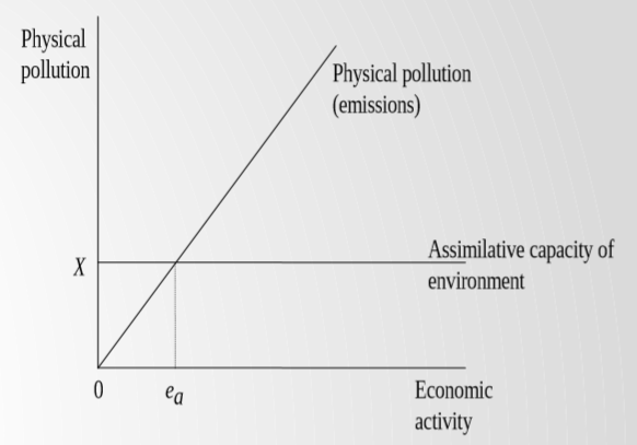
The pollution under x will be assimilated by the environment free of costs. Economic activity should be occurring as there is no negative effect to the environment.
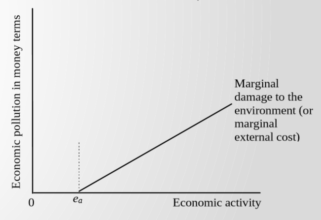
For ease, the vertical axis is shown in monetary cost of pollution.
The Marginal Damage (MD) is the amount of damage caused by an additional unit of pollution. Marginal damage increases as damage increases compared to pollution proportionally to the output. X-axis will either be labeled as economic activity or emissions of pollution.
Question: Do you think governments should force polluters to reduce their emissions to zero from an economic standpoint? There really is no reason to bring it to zero if the environment assimilates some waste without any damage.
Marginal Abatement Cost (MAC)
The cost of reducing one additional unit of pollutant is called the Marginal Abatement Cost (MAC). Both the MD and MAC curves are strictly convex. The implication of convex curves is that the total damage (measured with MAC as it is the cost of this damage) is increasing as economic activity increases, and MD is increasing as economic activity increases. A higher level of damage means that the marginal damage is higher and greater economic activity. The total abatement cost will increase with the level of abatement, and the marginal abatement cost increases with every unit abated.
It becomes more expensive to reduce emissions per extra unit
Application of standard marginal cost/ benefit equilibrium theory to pollution, but with marginal abatement cost / marginal damage (benefit comes from economic activity).
It becomes more expensive to reduce emissions by extra unit.
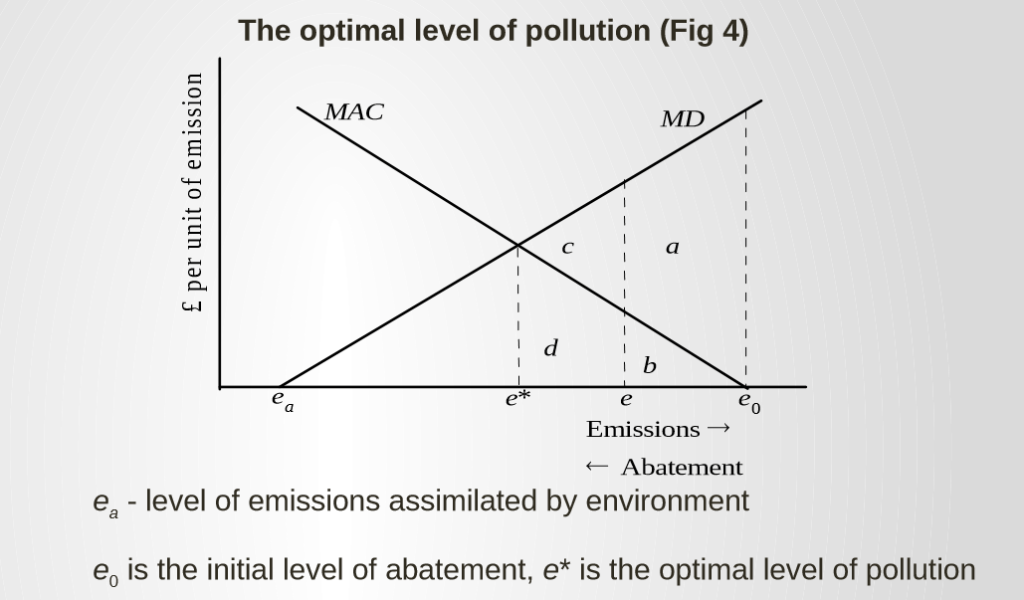
The area under the MAC is the total abatement cost. The area under the MD is the total damage caused by pollution. If emissions are reduced to a point e from e0, the total reduced damage will be a+b. This area is the reduced damage from the shift in emissions. Area a is the reduced damage due to less pollution emission, and area b is the reduced cost spent on abatement.
The welfare increase is area a, because it decreases the externality. Area b is just a reduction of the abatement cost for the industry or firm.
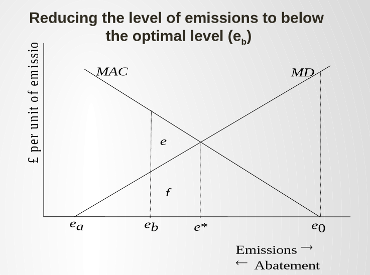
When emissions are reduced to below the optimal level, like for example to eb, the extra abatement cost is the area under MAC, so e and f. Area f is the increased welfare, as this is the area illustrating the decrease in emitted pollution in the industry. Area e is the increased abatement cost. The cost e is higher than the benefit f, so it is not beneficial to be at this emission level. It is not in our interest to lower the emission level below e*, which is the optimal level of pollution.
Focus of the module is on the right side of the diagram.
– End of the lecture on slide [14] –
